De Novo Design: Derivatives of Autoencoder

A primary goal of designing a deep learning architecture is to restrict the set of functions that can be learned to ones that match the **desired properties** from the domain
S Kearnes etal 2016 (Molecular Grpah Convolutions: Moving Beyond Fingerprints)
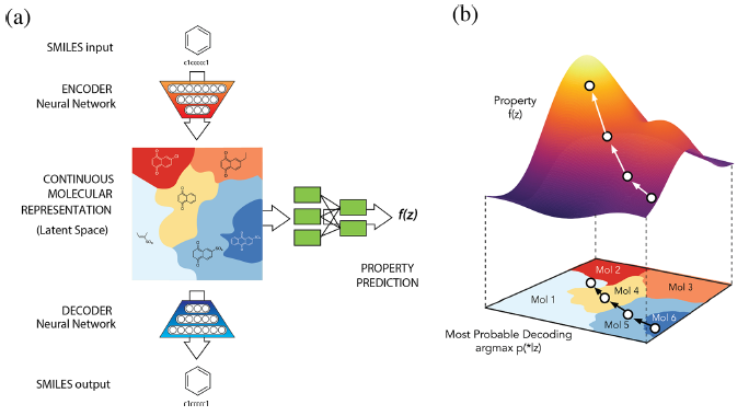
When building deep learning architecture, the above statement strongly highlights the key concept of implementing deep learning architecture. Especially, phrase “match the desired properties” can be understood as teaching, imposing a constraint, or regularization in several learning algorithm. For instance, GAN attempts to impose regularization by introducing Discriminator & Generator on the purpose of setting, and derivatives of Autoencoder predict a certain property by attaching MLP from latent space to get new datum with desired properties. Following takeaway outlines what I will illustrate in series with respect to generative models.
Structure of Generative Models
As Ian Goodfellow (NIPS 2014, and 2016 tutorial) demonstrates that maximizing Maximum Likelihood Estimates is equivalent to minimizing KL divergence between data generating distribution and the model and introduces Nash equilibrium, which verifies the unbiasness of GAN. On top of that, Generating a datum via Variational Autoencoder while simultaneously predicing property can be regarded as optimization with constraint. whether explicitily represent a probability distribution or not derives the fundamental difference between these two generative models(GAN & Variational Autoencoder).
Although the way of approach is different, convergence of disciplines such as Economcis, Industrial Engineering, Statistics, and Computer Science has appeared and they share the goal of implementing natural “regularization”.
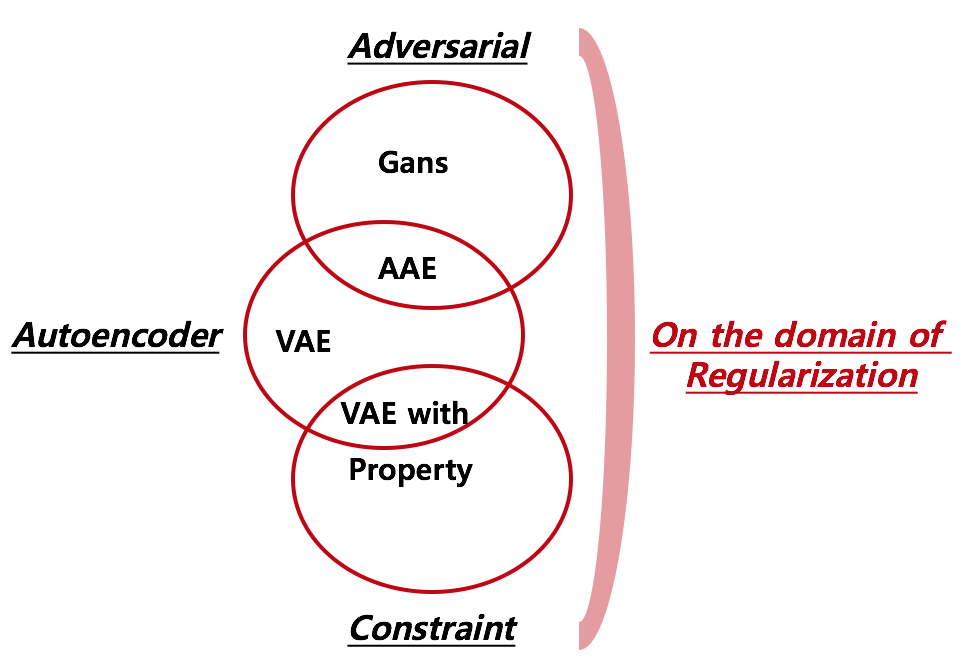
As for the widley known argloithm, foramts of regularization can be categorized into 2 folds: Game(Adversarial) and Predict property simultaneously(Constraint). By starting from the perspective of Autoencoder, I made 3 overlapping diagrams where “Adversarial” and “Constraint” lie on the domain of “regularization”.

1. Comparison of Models
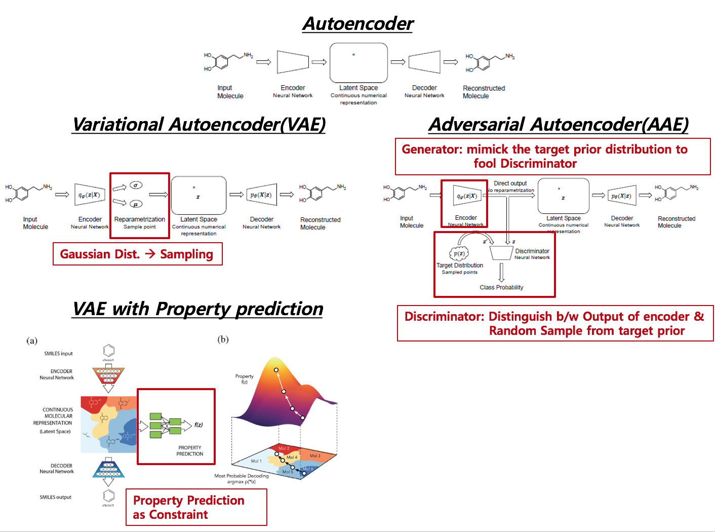
Below picture is combination of figures from different papers. Red box indicated in derivatives of autoencoder denotes different substructure across derivatives.

Distinctive Features across Methods
-
AE –> VAE Reparametrization from encoder to Latent Space via pre-assumed distribution (usually Gaussian distribtion)
-
VAE –> VAE with Property Added a netwrok from latent space to a supervised network such as Regression or Classification, which agglomerates Latent Space according to the level of target value.
-
AE –> AAE No Reparametrization, but adversarial Network is attached
Cost function across Methods
- AE : Reconstruction error
- VAE : Reconstruction error + KL-divergence (Regularizing Variational Parameter)
( latent space is driven by adding stochasticity to the encoder ) –> Adding noise to the encoded latent space forces the decoder to learn a wider range of latent points, which lead to find out more robust representations. - VAE with property: Reconstruction error of decoder + KL-divergence (Regularizing Variational Parameter) + regression error
- AAE : Reconstruction error of decoder + Discriminator loss + encoder(Generator) loss
In terms of regularizing the encoder posterior to match a pre-assumed prior, VAE with property and Adversarial autoencoder are on the same domain.
Specifically, Discriminator and Generator loss can be implemented like following
Discriminator related loss:

Generator related loss:

2. Data & Pre-processing
- Image or sequence (Molecular information is denoted as SMILES code, which is a sequence, will be mainly used )
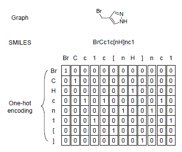
In this post, I will use data from Tox21 data and the input will be SMILES code, which is mainly used for chemical design and molecular property prediction. Data pre-processing and specific model illustration is described below ( reference: T Blaschke etal 2017 ).

To adopt periodic table into SMILES code, I merged chemical in periodic table with the code and generated one-hot encoded matrix for each SMILES code. Since the max length of chemical is 2, ismol variable in the function is
# tscode : SMILES code

# chnum  : Total unique number of chemcial in SMILES code considering periodic table

# ohlen  : Maximum number of SMILES code length (Usually restricted by researchers and users)


def onehot_encoder(tscode, chnum, ohlen):

    ohcode = np.zeros( ( chnum * ohlen ) )
    ohindex = 0
    mm = 0

    while   mm  < len( tscode )   :

        ch0 = tscode[ mm ]
        ismol = 0

        if ch0 in mcode   :
            ismol = 1

        if mm < len( tscode ) - 1 :

            ch1 = tscode[ mm + 1 ]
            if  ch0 + ch1 in mcode :
                ismol = 2
                mm = mm + 1

        if  ismol == 0 :
            ch = ch0
        elif ismol == 1 :
            ch = ch0
        elif ismol == 2 :
            ch = ch0 + ch1

        indx = codelist.index( ch )

        ohcode[ ohindex + indx ] = 1
        mm = mm + 1
        ohindex = ohindex + chnum

    return ohcode
3. Implementation of VAE with Proprty
3.1 HyperParameter Setting
import numpy                   as np
import pandas                  as pd
import tensorflow              as tf

# Convert smiles code into 2D array

import smiles_onehot_func      as sof


from   math                    import ceil
from   datetime                import datetime

from   rdkit.Chem              import MolFromSmiles
from   rdkit.Chem.QED          import qed
from   rdkit.Chem.Descriptors  import MolWt
from   rdkit                   import DataStructs
from   rdkit.Chem.Fingerprints import FingerprintMols

scode = sof.trX

ver_str       = "v1.1.3"

# GPU allocation

gpu_num       = str( 0 )

learning_rate = 0.0001
num_epoch     = 1000
num_rs        = 5000
batch_size    = 50
print_time    = 10
save_epoch    = 10

# Latent Space dimension in AE

latent_dim    = 1024

# Latent Space dimension in VAE (latent dim --> variational_dim via Reparametrization trick)

variation_dim = 256

# 2D array dimension

ohlen         = sof.m_ohlen
chnum         = sof.m_chnum

# Convolution nodes

num_clayer1   = 64
num_clayer2   = 128

ol_devide_2   = ceil( ohlen       / 2 )
ol_devide_4   = ceil( ol_devide_2 / 2 )

cl_devide_2   = ceil( chnum       / 2 )
cl_devide_4   = ceil( cl_devide_2 / 2 )


# Placeholders for Input and target

x         = tf.placeholder( tf.float32, [ None, ohlen, chnum,  1 ], name="input"  )
label     = tf.placeholder( tf.float32, [ None, ohlen, chnum,  1 ], name="label"  )

latent    = tf.placeholder( tf.float32, [ None, variation_dim       ], name="latent" ) #latent space  at VAE


prop      = tf.placeholder( tf.float32, [ None, 1                ], name="prop"   ) # regression target value


# Variational Parameters

weights = {
    'z_mean': tf.Variable(tf.truncated_normal([latent_dim, variation_dim])),
    'z_std': tf.Variable(tf.truncated_normal([latent_dim, variation_dim]))
}

biases = {
    'z_mean': tf.Variable(tf.zeros([variation_dim])),
    'z_std': tf.Variable(tf.zeros([variation_dim]))
}
3.2 Encoder
def encoder( inputs, is_training ) :

    # === Convoltion Sets

    conv1     = tf.layers.conv2d( inputs = inputs,   filters = num_clayer1, kernel_size = ( 3, 3 ), padding = 'same', activation = None )
    conv1     = tf.layers.batch_normalization( conv1, center = True, scale = True, training = is_training )
    conv1     = tf.nn.relu( conv1 )
    maxpool1  = tf.layers.max_pooling2d( conv1, pool_size = ( 2, 2 ), strides = ( 2, 2 ) , padding = 'same' ) # 50 x 71


    conv2     = tf.layers.conv2d( inputs = maxpool1, filters = num_clayer2, kernel_size = ( 3, 3 ), padding = 'same', activation = None )
    conv2     = tf.layers.batch_normalization( conv2, center = True, scale = True, training = is_training )
    conv2     = tf.nn.relu( conv2 )
    maxpool2  = tf.layers.max_pooling2d( conv2, pool_size = ( 2, 2 ), strides = ( 2, 2 ) , padding = 'same' ) # 25 x 36

    maxpool2  = tf.reshape( maxpool2, [ - 1, ol_devide_4 * cl_devide_4 * num_clayer2 ] )

    encoded   = tf.layers.dense( inputs = maxpool2, units = latent_dim, activation = None )
    encoded   = tf.layers.batch_normalization( encoded, center = True, scale = True, training = is_training )
    encoded   = tf.nn.relu( encoded, name = "encoded" )

    # === ADD VARIATIONAL

    z_mean    = tf.matmul(encoded, weights['z_mean']) + biases['z_mean']
    z_std     = tf.matmul(encoded, weights['z_std']) + biases['z_std']
    z_std     = 1e-6 + tf.nn.softplus( z_std )

    # === Reparametrization

    z         = z_mean + z_std * tf.random_normal(tf.shape(z_mean), 0, 1, dtype=tf.float32)

    return z , z_mean, z_std
3.3 Decoder
def decoder( encoded, is_training ) :

    # === DeConvoltion Sets (More or less Upsampling)

    fullcon   = tf.layers.dense( inputs = encoded,  units = ol_devide_4 * cl_devide_4 * num_clayer2, activation = None )
    fullcon   = tf.layers.batch_normalization( fullcon, center = True, scale = True, training = is_training )
    fullcon   = tf.nn.relu( fullcon )
    fullcon   = tf.reshape( fullcon, [ - 1, ol_devide_4, cl_devide_4, num_clayer2 ] )

    upsample1 = tf.image.resize_images( fullcon, size = ( ol_devide_2, cl_devide_2 ), method = tf.image.ResizeMethod.NEAREST_NEIGHBOR )
    conv4     = tf.layers.conv2d( inputs = upsample1, filters = num_clayer2, kernel_size = ( 3, 3 ), padding = 'same', activation = None )
    conv4     = tf.layers.batch_normalization( conv4, center = True, scale = True, training = is_training )
    conv4     = tf.nn.relu( conv4 )

    upsample2 = tf.image.resize_images( conv4,   size = ( ohlen, chnum ), method = tf.image.ResizeMethod.NEAREST_NEIGHBOR )
    conv5     = tf.layers.conv2d( inputs = upsample2, filters = num_clayer1, kernel_size = ( 3, 3 ), padding = 'same', activation = None )
    conv5     = tf.layers.batch_normalization( conv5, center = True, scale = True, training = is_training )
    conv5     = tf.nn.relu( conv5 )

    logits    = tf.layers.conv2d( inputs = conv5,     filters =  1, kernel_size = ( 3, 3 ), padding = 'same', activation = None )
    logits    = tf.add( logits, 0.0, name = "decoded" )

    return logits
3.4 Regression
def property_regression( encoded ) :

    fullcon1   = tf.layers.dense( inputs = encoded , units = 512, activation = None )
    fullcon1   = tf.nn.relu( fullcon1 )

    fullcon2   = tf.layers.dense( inputs = fullcon1, units = 512, activation = None )
    fullcon2   = tf.nn.relu( fullcon2 )

    output     = tf.layers.dense( inputs = fullcon2, units = 1  , activation = tf.nn.sigmoid )
    output     = tf.add( output, 0, name = "property" )

    return output
3.5 VAE Loss
def vae_loss(x_reconstructed, x_true, z_mean, z_std ):

    # === Reconstruction loss

    marginal_likelihood = tf.reduce_sum(tf.nn.sigmoid_cross_entropy_with_logits( logits=x_reconstructed, labels=x_true), axis=1)

    # === VAE loss from another script file


    KL_divergence = 0.5 * tf.reduce_sum(tf.square(z_mean) + tf.square(z_std) - tf.log(1e-8 + tf.square(z_std)) - 1, 1)

    marginal_likelihood = tf.reduce_mean(marginal_likelihood)
    KL_divergence = tf.reduce_mean(KL_divergence)

    loss = marginal_likelihood + KL_divergence

    return loss, marginal_likelihood, KL_divergence
3.6 Training
def train( re_training = False ) :

    # === Collect Variables via scope


    with tf.variable_scope("AE"):
        z, z_mean, z_std  = encoder( x      , is_training = True )
        logits                  = decoder( z, is_training = True )

    with tf.variable_scope( "FC" ) :
        prop_reg  = property_regression( z )

    # === VAE loss

    loss_ae , NML, KL  = vae_loss( logits, label, z_mean, z_std )

    # === Regression loss

    loss_fc   = tf.reduce_mean( tf.losses.mean_squared_error( labels = prop, predictions = prop_reg ) )

    # === get variable for each model

    t_vars    = tf.trainable_variables( ) # return list

    en_vars   = [ var for var in t_vars if "AE" in var.name ]

    # === Cost function

    cost_ae   = tf.add( loss_ae, 0, name = "cost_ae" )
    cost_all   = tf.add( cost_ae, loss_fc, name = "cost_all" )

    # === Recall Batch Normalization in VAE

    update_ops_en = tf.get_collection( tf.GraphKeys.UPDATE_OPS, scope = "AE" )

    # === Optimization

    optimizer     = tf.train.AdamOptimizer( learning_rate )

    with tf.control_dependencies( update_ops_en ):
        optimizer_ae = optimizer.minimize( cost_all, var_list = en_vars, name = "optimizer_ae" )

    init      = tf.global_variables_initializer( )
    saver     = tf.train.Saver( )


    c = tf.ConfigProto()
    c.gpu_options.visible_device_list = gpu_num

    with tf.Session( config = c ) as sess :

        sess.run( init )

        if re_training :
            saver.restore( sess, save_path = tf.train.latest_checkpoint( model_path ) )
            last_epoch = tf.train.latest_checkpoint( model_path ).split( "-" )[ - 1 ]


        for epoch in range( num_epoch ) :

            if re_training :
                if epoch < int( last_epoch ) :
                    print( "skip epoch {}...".format( epoch ) )
                    continue

            for i in range( num_rs ) :

                batch, props = sof.GetOnehotBatch( batch_size )
                imgs         = batch.reshape( [ - 1, ohlen, chnum, 1 ] )

                cs_ae, cs_nml, cs_kl, cs_fc, _ = sess.run( [ cost_ae, NML, KL ,loss_fc, optimizer_ae ],
                                                         feed_dict={ x : imgs, label : imgs, prop : props } )

                if i % print_time == 0 :
                    print( ver_str + "      Max Length : " + str( ohlen ) + "      Using GPU : " + gpu_num )

                    print( "Epoch : {}/{}  iter : {}/{}...".format( epoch + 1, num_epoch, i + 1, num_rs ) + "\n" +
                           "VAE loss : {:.6f}    ".format( cs_ae )              +
                           "NML loss : {:.6f}     ".format( cs_nml )              +
                           "KL loss : {:.6f}     ".format( cs_kl )              +
                           "    Prop Regression loss : {:.6f}".format( cs_fc )  +
                           "    duration time : " + str( t4 - t3 )

            if ( epoch + 1 ) % save_epoch == 0 :
                saver.save( sess, model_path, global_step = ( epoch + 1 ) )

        saver.save( sess, model_path, global_step = ( epoch + 1 ) )
Reference
-
Kearnes, Steven, et al. “Molecular graph convolutions: moving beyond fingerprints.” Journal of computer-aided molecular design 30.8 (2016): 595-608.
-
Blaschke, Thomas, et al. “Application of generative autoencoder in de novo molecular design.” Molecular informatics 37.1-2 (2018).
-
Gómez-Bombarelli, Rafael, et al. “Automatic chemical design using a data-driven continuous representation of molecules.” ACS Central Science 4.2 (2018): 268-276.
-
Goodfellow, Ian, et al. “Generative adversarial nets.” Advances in neural information processing systems. 2014.
-
Github of VAE with property prediction : Chemical VAE

