Multi-Column Deep Neural Network
Motivation of implementing MCDNN for Image classification
The thing I would like to remind myself is that most of real world data is totally different from MNIST or CIFAR10 in terms of standardization. Suppose your images are generated by a sensor machine through automatic object detection. Since the machine captures an object with a certain degree of freedom, the size of an image, location of an object, and lightness of background might be variant across time and classes. Even the camera and scope of an object are fixed, diverse image pre-processing can affect the model accuracy. In addition, weighted voting or averaging different CNN models has possibility of improving the model performance. As a way to merge such possibilities, Ciresan etal 2012, CVPR Multi-Column Deep Neural Network (MCDNN), which is an ensemble of CNNs can be applied. This paper argues that combining multiple CNNs and averaging the output score can boost the prediction accuracy with low error rate.
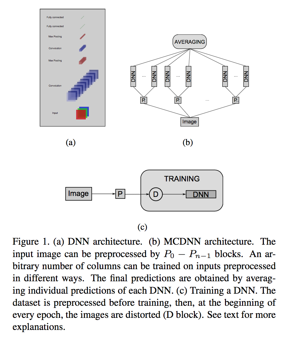
Illustration image from Ciresan etal 2012 CVPR
Project issues
Image data in one of my multi-classification task has high complexity with overlapping features across classes, which makes it difficult to draw decision borders with a single combination of pre-processing and model, so I applied main concept of MDCNN on multi-classification within the limit of GPU capability(GeForce 1080Ti 11G). Below, I posted a class object that I used to generate multiple graphs and sessions for the training and testing by python & Tensorflow.
Class for declaring multiple graphs and sessions
# Initial Set Up

config = tf.ConfigProto()
config.gpu_options.per_process_gpu_memory_fraction = 0.8

param_path = '/path/to/saved/parameter'


NN = 24

class graph_sess(object):

    def __init__(self, N, param_path):

        self.N = N
        self.param_path = param_path

    def graph(self):

        d = collections.OrderedDict()

        for x in range(N):
            if x < 10:
                d["g0{0}".format(x)] = tf.Graph()
            else:
                d["g{0}".format(x)] = tf.Graph()

        return list(d.items())

    def session(self):

        item_res = self.graph()

        for i in range(self.N):

            with item_res[i][1].as_default():

                if i < 10:
                    index = "0{0}".format(i)
                else:
                    index = "{0}".format(i)

                globals()['sess%s' % index] = tf.Session(config=config)

                globals()['saver%s' % index] = tf.train.import_meta_graph(self.param_path + 'model.meta')
                globals()['saver%s' % index].restore(globals()['sess%s' % index], self.param_path + 'model')

                tf.get_default_graph().as_graph_def()

                globals()['x%s' % index] = globals()['sess%s' % index].graph.get_tensor_by_name("input:0")
                globals()['y%s' % index] = globals()['sess%s' % index].graph.get_tensor_by_name("output:0")

                # Depending on the CNN structure, change the dropout or other options.
                globals()['kp1%s' % index] = globals()['sess%s' % index].graph.get_tensor_by_name("keep_prob1:0")
                globals()['kp2%s' % index] = globals()['sess%s' % index].graph.get_tensor_by_name("keep_prob2:0")
                globals()['kp3%s' % index] = globals()['sess%s' % index].graph.get_tensor_by_name("keep_prob3:0")
                globals()['ys%s' % index] = tf.nn.softmax(globals()['y%s' % index])
                globals()['cr%s' % index] = tf.argmax(globals()['ys%s' % index], 1)


graph_sess_inst = graph_sess(NN, param_path)
graph_sess_inst.session()
Wrap-up
There are sill several issues regarding how to implement combinations of pre-processing and CNN Models. For instance, image pre-processing can have different options like inner padding, zero-padding, and edge filter. Also, the architecture of CNNs can be various through the number of hidden layer, kernel size, and the existence of pooling layer. Lastly, different ways of merging multiple outputs should be considered. Basically, we are able to average outcomes as in the paper or weighted voting. Attacking theses issues will be adjusted by data and project goals.
Recommendation System by Siamese Network
Recommendations using triplet loss
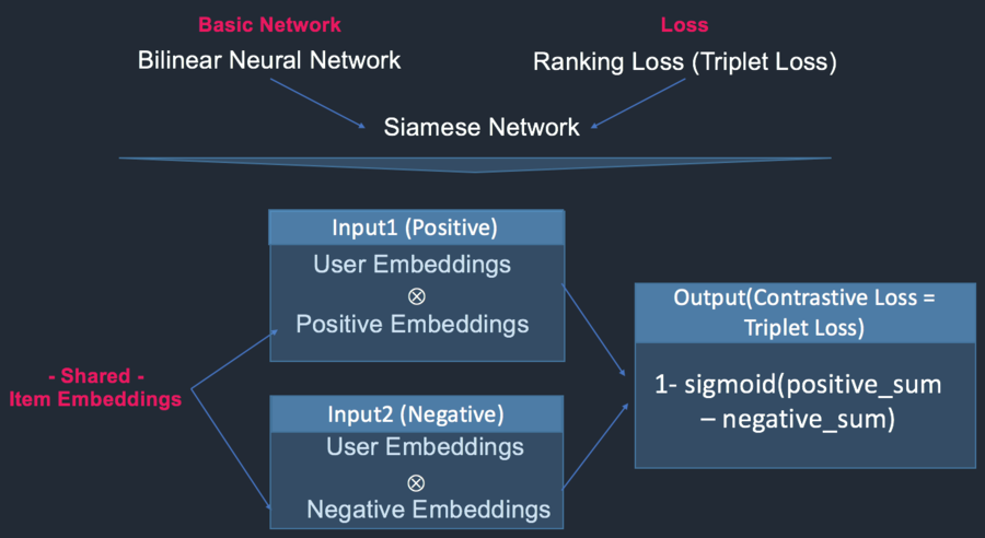
When both positive and negative items are specified by user, recommendation based on Siamese Network can account such preference and rank positive items higher than negative items. To implements this, I transformed maciej’s github code to account for user specific negative preference. Just as word2vec idea (matrix multiplication that transforms words into corresponding word embeddings), latent factor matrix can be represented by embedding layers. The original idea is building Bilinear Neural Network and Ranking Loss(Triplet Loss), and combine them into Siamese Network architecture siames_blog. The triplet is user, positive items, and negative items.
The below picture demonstrates the way to construct the architecture. Positive and negative item embeddings share a item embedding layer, and each of them are multiplied by a user embedding layer. Although the original code used Movielens100k dataset and randomly selects negative items randomly, which can lead negative items to contain some positive items, I set the negative items with score less than 2 and positive items greater than 5.
Since negative and positive embedding layers share the same item embedding layer, the size of them should be equal. To suffice the deficient amount of negative items, I randomly select items from the recordings 3 and put them into negative items. Finally, The network is built upon Keras backedn Tensorflow. The final outcomes with 20 epcoh shows 82% of AUC(Area Under Curve of ROC curve).
Specific implementation
Data import
import numpy as np
import itertools
import os
import requests

import zipfile
import scipy.sparse as sp
from sklearn.metrics import roc_auc_score

def download_movielens(dest_path):

    url = 'http://files.grouplens.org/datasets/movielens/ml-100k.zip'
    req = requests.get(url, stream=True)

    with open(dest_path, 'wb') as fd:
        for chunk in req.iter_content():
            fd.write(chunk)

def get_raw_movielens_data():

    path = '/path/to/data/saved/movielens.zip'

    if not os.path.isfile(path):
        download_movielens(path)

    with zipfile.ZipFile(path) as datafile:
        return (datafile.read('ml-100k/ua.base').decode().split('\n'),
                datafile.read('ml-100k/ua.test').decode().split('\n'))
Data Pre-Processing
def parse(data):

    for line in data:

        if not line:
            continue

        uid, iid, rating, timestamp = [int(x) for x in line.split('\t')]

        yield uid, iid, rating, timestamp

def build_interaction_matrix(rows, cols, data):

    mat_pos = sp.lil_matrix((rows, cols), dtype=np.int32)
    mat_neg = sp.lil_matrix((rows, cols), dtype=np.int32)
    mat_mid = sp.lil_matrix((rows, cols), dtype=np.int32)

    for uid, iid, rating, timestamp in data:

        if rating >= 5.0:
            mat_pos[uid, iid] = 1.0

        elif rating <= 2.0:
            mat_neg[uid, iid] = 1.0

        elif rating == 3.0:
            mat_mid[uid, iid] = 1.0

    possum = mat_pos.sum(); negsum = mat_neg.sum();

    # Sampling negative index not included from positive & negatively indicated one

    # Sampling deficient amount from the mat_mid value == 1
    b = mat_mid.toarray() == 1.0
    index = np.column_stack(np.where(b))

    # Shuffle allindex and get the first N(deficient) amount location
    np.random.shuffle(index)

    if negsum < possum:

        deficient = (possum - negsum)
        allindex = index[:deficient, ]

        # Asgign value into mat_neg where mat_mid occurs
        for idx, val in enumerate(allindex):
            mat_neg[val[0] , val[1]] = 1.0

        possum = mat_pos.sum(); negsum = mat_neg.sum()

        if possum != negsum:
            print("Number of Positive and negative doesn't match!!")
            pass


    elif possum > negsum:

        deficient = (negsum - possum)
        allindex = index[:deficient, ]

        # Asgign value into mat_neg where mat_mid occurs
        for idx, val in enumerate(allindex):
            mat_pos[val[0], val[1]] = 1.0

    return ( mat_pos.tocoo(), mat_neg.tocoo() )


def get_movielens_data():

    train_data, test_data = get_raw_movielens_data()

    uids = set()
    iids = set()

    for uid, iid, rating, timestamp in itertools.chain(parse(train_data),parse(test_data)):
        uids.add(uid)
        iids.add(iid)

    rows = max(uids) + 1
    cols = max(iids) + 1

    train_pos , train_neg = build_interaction_matrix(rows, cols, parse(train_data))
    test_pos , test_neg = build_interaction_matrix(rows, cols, parse(test_data))

    return (train_pos , train_neg, test_pos , test_neg)
Keras Model Implementation
from keras import backend as K
from keras.models import Model, Sequential
from keras.layers import Embedding, Flatten, Input, Convolution1D ,merge
from keras.optimizers import Adam

def bpr_triplet_loss(X):

    positive_item_latent, negative_item_latent, user_latent = X

    # BPR loss
    loss = 1.0 - K.sigmoid(
        K.sum(user_latent * positive_item_latent, axis=-1, keepdims=True) -
        K.sum(user_latent * negative_item_latent, axis=-1, keepdims=True))

    return loss

def identity_loss(y_true, y_pred):

    return K.mean(y_pred - 0 * y_true)


def build_model(num_users, num_items, latent_dim):

    # Input
    positive_item_input = Input((1, ), name='positive_item_input')
    negative_item_input = Input((1, ), name='negative_item_input')

    user_input = Input((1, ), name='user_input')

    # Embedding
    # Shared embedding layer for positive and negative items
    item_embedding_layer = Embedding( num_items, latent_dim, name='item_embedding', input_length=1)

    positive_item_embedding = Flatten()(item_embedding_layer(positive_item_input))
    negative_item_embedding = Flatten()(item_embedding_layer(negative_item_input))

    user_embedding = Flatten()(Embedding( num_users, latent_dim, name='user_embedding', input_length=1)(user_input))

    # Loss and model
    loss = merge(
        [positive_item_embedding, negative_item_embedding, user_embedding],
        mode=bpr_triplet_loss,
        name='loss',
        output_shape=(1, ))

    model = Model(
        input=[positive_item_input, negative_item_input, user_input],
        output=loss)

    model.compile(loss=identity_loss, optimizer=Adam())

    return model
Divide&Conquer on CNN
Image Classification by Divide & Conquer
Although classifying MNIST data can be achieved with small convolution set because of distinctive features for each class, lots of projects are relatively more complicated. Suppose your mission is on distinguishing images into 2 classes, while the difference between 2 images is little, ambiguous, and extensively distributed across regions. Applying CNN into an entire image is likely to crush subtle difference between 2 classes. One of the possible solutions to attack this problem is to train separate CNN for a grid of sliced image. In other words, divide a classification problem into multiple sub-problems and generate multiple sub-solution. combining sub-solution will make a concrete result for the classification of an image.
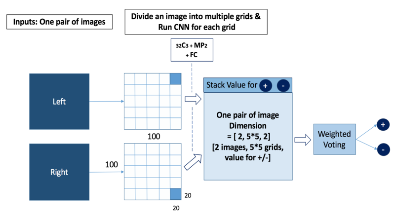
In tensorflow, you can generate multiple weights and bias for each grid of an image like this.
Generate multiple Grids of an image
# Divide an image by shape of a grid
def blockshaped(arr, nrows, ncols):
    h, w = arr.shape
    return (arr.reshape(h//nrows, nrows, -1, ncols)
               .swapaxes(1,2)
               .reshape(-1, nrows, ncols))
Functions generating weights and bias
# Weight and Bias for one grid CNN and FC

def variable_generate():
    w_conv1 = weight_variable( [ 3, 3, 1, 32 ] )
    b_conv1 = bias_variable( [ 32 ] )

    w_fc1 = weight_variable( [ 25 * 25 * 32,  64] )
    b_fc1 = bias_variable( [ 64 ] )

    w_out1 = weight_variable([64,2])

    return w_conv1, b_conv1, w_fc1, b_fc1, w_out1


# Variables for each grid of an image

N = 25
weights={}
for x in range(0,N):

    w_conv, b_conv, w_fc, b_fc, w_out = variable_generate()
    weights["w_conv{0}".formt(x)] = w_conv
    weights["b_conv{0}".formt(x)] = b_conv
    weights["w_fc{0}".formt(x)] = w_fc
    weights["b_fc{0}".formt(x)] = b_fc
    weights["w_out{0}".formt(x)] = w_out
Classification_Result
Classification with Fuzzy system Part2 (Result)
Basically, this post is about how to wrap up the results from training classification with Fuzzy system by Gaussian pdf with different standard deviation. I will illustrate how standard deviation in Multivariate Gaussian pdf generates different prediction(max position) and mean value across output nodes. The visualization of the summary result will be based on the fitted value(good and inferior product images) and prediction(unknown images) since I trained the model with respect to good and inferior images.
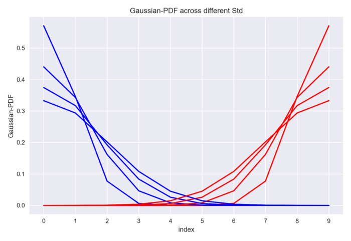
Different standard deviation(I assumed covariance matrix as std * Identity matrix) in Multivariate Gaussian across ratings can be displayed like the above. Since I will use half of Gaussian distribution with mutually exclusive classes and cross-entropy as a cost function, I set up the sum of pdf equals 1 and each probability value is between 0 and 1(for sure). Although softmax function will satisfy those two criteria, I pre-adjust the settings. On the purpose of grading , the average value across 10 output nodes is used here because it provides the degree of goodness and inferiority.
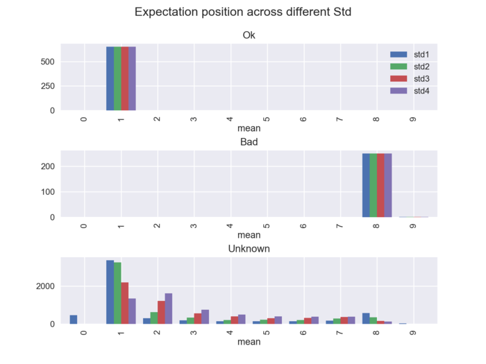
To validate the model, I made a bar plot for the max position(prediction) and mean position(expectation) of 10 output nodes grouped by different Std. With respect to fitted value(good and bad images), the result shows that the model is quite-well trained in terms of max and mean position. For prediction(Unknown images), the higher Std, the more images are distributed across ratings.
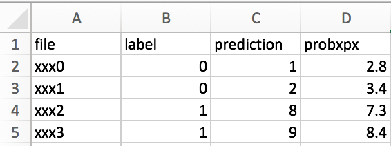
Moreover, to check how each image is predicted from different std model, I produced a CSV file containing each value (mean position or max position) across the different std and measure the std of the each value across different model. This procedure enables us to suggest suspicious images and request confirmation for the label of images to engineers.

Classification_FuzzySystem
Classification with Fuzzy system
To escape the possibility of label inaccuracy, I introduced not [0, 1], but the pdf with 10 density(Fuzzy system). Applying PDF for the class label will not only lead data scientist to resolve inaccuracy of data label but also empower themselves to suggest ratings of a product by maximum value with probability and average score.
Contents
Modification: Only training code will be left here.
0. Convert label to fuzzy system
1. Import images and balance batches
2. Train module
3. Test module
4. Unknown labeled images validation - skip
0.Fundamental tweak - Replacement of integer by fuzzy system
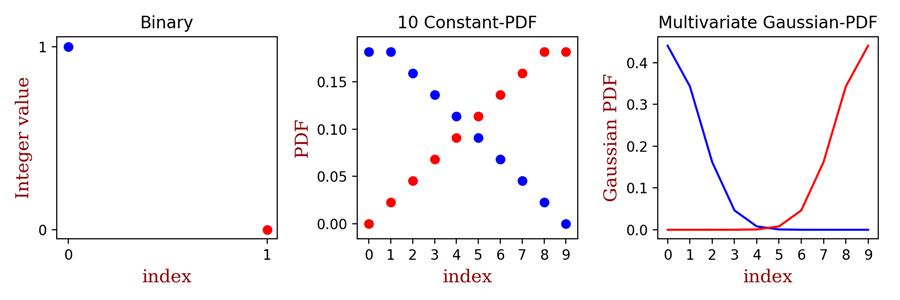
The traditional way of labeling an image for binary classification is to set 0 for + and 1 for -. However, in the case of deciding goodness of a product by image, such way can’t suggest the degree of goodness and badness. In addition, it’s difficult to apply such classification method when the label is indefinite. To overcome such limitations, I generate 10 output labels, where each of them is actually pdf, and the pdf value decreases as the further from the focal location with a constant interval. Such PDF(Probability Density Function) can be replaced with Gaussian, Exponential, or gamma distribution. Setting PDF, which takes on continuous values between 0 and 1, is called “Fuzzy system”. Below graph illustrates how different fuzzy system from the setting of an integer value.
Although I analyzed how unknown labeled images are classified and validate them with functions that I made, I will skip it here. Please email me if you are interested in it.
Although lots of examples for CNN with MNIST data uses one-hot-encoding labels, a little tweak on setting label can change it as the fuzzy system like this.
# Folder name starts with ‘o’ indicates + and with ‘b’ indicates - .

if filename ==‘o’:
	label = np.array( [1, 1, 0.875, 0.75, 0.625, 0.5, 0.375, 0.250, 0.125, 0 ] ) / 5.5
if filename ==‘b’
	label = np.array( [0, 0.125, 0.250, 0.375, 0.5, 0.625, 0.75, 0.875, 1, , 1 ] ) / 5.5
1.1 Batch specifications from +/-
My task was to import image data labeled as +/-. On the purpose of balancing the amount of +/- images in a batch, I generate the batch to comprise half of each +/- image. To ensure data randomization, I shuffled each +/- images after an epoch. In addition, if an index for the batch list is out of list size, my code will insert the rest of images and add them from the start of the list. Finally, since the number of +/- images are different in my project, I made this procedure work separately for each +/- images.
1.2 Convert images
In terms of generating images from the batch, I first resize images according to the normal ratio of original images(width/height) and interpolate them using nearest resample method, which can keep the information of images. Using like “PIL.Image.ANTIALIAS”, which is widely applicable in Photoshop, will smooth images and result in losing information of images. To implement this module, save the below script as makebatch.py.
2. Train module
After importing a batch, the CNN model is a convolution set (32C16 + MP2) with MLP2. The 32C16 indicates 32 neurons and the size of each neuron is 16 by 16. MP2 is for max pooling with stride 2. Finally, MLP2(Multi-Layer Perceptron) is for the fully connected layer with 2 hidden layers.
import matplotlib.pyplot as plt
import numpy as np
from PIL import Image
from datetime import datetime
## get all filelist
import os
from os import listdir
from os.path import isfile, join

# import makebatch modul, which is written above

import makebatch
batch = makebatch.Batch()


###################################### Classification ########################\
import tensorflow as tf
sess = tf.InteractiveSession()

# x : input image /  y_
x = tf.placeholder(tf.float32, shape=[None, 512*64], name = "input")
y = tf.placeholder(tf.float32, shape=[None, 10])

### Convolution Neural Network

def weight_variable(shape):
    initial = tf.truncated_normal(shape, stddev=0.1)
    return tf.Variable(initial)

def bias_variable(shape):
    initial = tf.constant(0.1, shape=shape)
    return tf.Variable(initial)

def conv2d(x, W):
    return tf.nn.conv2d(x, W, strides=[1, 1, 1, 1], padding='SAME')

def max_pool_2x2(x):
    return tf.nn.max_pool(x, ksize=[1, 2, 2, 1], strides=[1, 2, 2, 1], padding='SAME')


#convolution & pooling 1
x_image = tf.reshape( x, [ -1, 512, 64, 1 ] )

W_conv1 = weight_variable( [ 16, 16, 1, 32 ] )
b_conv1 = bias_variable( [ 32 ] )

h_conv1 = tf.nn.relu( conv2d( x_image, W_conv1 ) + b_conv1 )
h_pool1 = max_pool_2x2( h_conv1 )

#fully connected 1
h_pool2_flat = tf.reshape( h_pool1, [ -1, 256 * 32 * 32 ] )

W_fc1 = weight_variable( [256 * 32  * 32 , 256 ] )
b_fc1 = bias_variable( [ 256 ] )

h_fc1 = tf.nn.relu( tf.matmul( h_pool2_flat, W_fc1 ) + b_fc1 )

W_fc2 = weight_variable([256, 10])
b_fc2 = bias_variable([10])

y_conv = tf.add(tf.matmul(h_fc1, W_fc2), b_fc2, name = "output")

cross_entropy = tf.reduce_mean(tf.nn.softmax_cross_entropy_with_logits(labels=y, logits=y_conv))
train_step = tf.train.AdamOptimizer(1e-4).minimize(cross_entropy)
correct_prediction = tf.equal(tf.argmax(y_conv,1), tf.argmax(y,1))
accuracy = tf.reduce_mean(tf.cast(correct_prediction, tf.float32))
sess.run(tf.global_variables_initializer())


saver = tf.train.Saver()

costlist0 = []; acculist0 = [];
for epoch in range(150):

    costlist1 =[]; acculist1 = [];
    for i in range( 130 ):

        iter1start = datetime.now()

        file0 = batch.indexing(10)
        trX , trY = makebatch.datagenerate(file0)


        if i%1== 0:
            print("%d epoch %d th iteration..."%( epoch+1, i ) )

        c = sess.run(cross_entropy, feed_dict={x: trX, y: trY})
        costlist1.append(c)
        print("cost is %f:  "  %c)

        train_step.run(feed_dict={x: trX, y: trY})

        #accu = sess.run(accuracy, feed_dict={x: trX, y: trY})
        #print("accuracy is %f:  "  %accu)
        #acculist1.append(accu)

        batch.next_batch()

        iter1end = datetime.now()
        iter1time = iter1end - iter1start
        print("iteration 1 running time: " + str(iter1time) )
    costlist0.append(costlist1)
    acculist0.append(acculist1)

saver.save(sess, "path/to/save/model/model")