Self-Organizing-MAP with MNIST data
Self-Organizing-MAP(SOM)
Suppose your mission is to cluster colors, images, or text. Unsupervised learning(no label information is provided) can handle such problems, and specifically for image clustering, one of the most widely used algorithms is Self-Organizing-MAP(SOM).
The ‘Map’ of SOM indicates the locations of neurons, which is different from the neuron graph of Artificial Neural Network(ANN). Based on this ‘locations’, SOM presumes that closely connected neurons and inputs share similar properties. Such closest neuron is denoted as Best Matching Unit(BMU), and calculated based on the Euclidean distance between the neuron and inputs. The below figure demonstrates a small network of 5*4 neurons. For each iteration, after BMU is determined, SOM calculates the weights of other units within BMU’s neighborhood(the size of the initial neighborhood is pre-determined). As iteration number increases, the length of neighborhood radius and learning rate can be set up to decrease.

Specific Algorithm
-
Once each neuron’s weights are initialized, every neuron is examined to calculate the distance to inputs(the length of inputs should be the same as that of neuron weights in order to calculate the distance).
-
A neuron that has the smallest distance will be chosen as Best Matching Unit(BMU) - aka winning neuron.
-
The radius of a neighborhood of the BMU starts from the specified value and shrinks as the iteration increases. Found Nodes inside of the neighborhood are getting similar by changing their weights
SOM with MNIST data
Sachin Joglekar’s blog has illustrated how SOM algorithm works and its implementation in Tensorflow. I will apply a little-modified class ‘SOM’ into MNIST data and examine how well SOM works.
import matplotlib.pyplot as plt
import numpy as np
import random as ran

## Applying SOM into Mnist data

from tensorflow.examples.tutorials.mnist import input_data
mnist = input_data.read_data_sets("MNIST_data", one_hot=True)

def train_size(num):
    x_train = mnist.train.images[:num,:]
    y_train = mnist.train.labels[:num,:]
    return x_train, y_train

x_train, y_train = train_size(100)
x_test, y_test = train_size(110)
x_test = x_test[100:110,:]; y_test = y_test[100:110,:]

def display_digit(num):
    label = y_train[num].argmax(axis=0)
    image = x_train[num].reshape([28,28])
    plt.title('Example: %d  Label: %d' % (num, label))
    plt.imshow(image, cmap=plt.get_cmap('gray_r'))
    plt.show()

display_digit(ran.randint(0, x_train.shape[0]))

# Import som class and train into 30 * 30 sized of SOM lattice
from som import SOM

som = SOM(30, 30, x_train.shape[1], 200)
som.train(x_train)

# Fit train data into SOM lattice
mapped = som.map_vects(x_train)
mappedarr = np.array(mapped)
x1 = mappedarr[:,0]; y1 = mappedarr[:,1]

index = [ np.where(r==1)[0][0] for r in y_train ]
index = list(map(str, index))

## Plots: 1) Train 2) Test+Train ###

plt.figure(1, figsize=(12,6))
plt.subplot(121)
# Plot 1 for Training only
plt.scatter(x1,y1)
# Just adding text
for i, m in enumerate(mapped):
    plt.text( m[0], m[1],index[i], ha='center', va='center', bbox=dict(facecolor='white', alpha=0.5, lw=0))
plt.title('Train MNIST 100')

# Testing
mappedtest = som.map_vects(x_test)
mappedtestarr = np.array(mappedtest)
x2 = mappedtestarr[:,0]
y2 = mappedtestarr[:,1]

index2 = [ np.where(r==1)[0][0] for r in y_test ]
index2 = list(map(str, index2))

plt.subplot(122)
# Plot 2: Training + Testing
plt.scatter(x1,y1)
# Just adding text
for i, m in enumerate(mapped):
    plt.text( m[0], m[1],index[i], ha='center', va='center', bbox=dict(facecolor='white', alpha=0.5, lw=0))

plt.scatter(x2,y2)
# Just adding text
for i, m in enumerate(mappedtest):
    plt.text( m[0], m[1],index2[i], ha='center', va='center', bbox=dict(facecolor='red', alpha=0.5, lw=0))
plt.title('Test MNIST 10 + Train MNIST 100')

plt.show()
Each of the plotted MNIST test digits is well fitted into the target locations! Although digit 3 and 5 are not completely split, it seems to be resolved if the number of training iteration increases.
Within the SOM class written by Sachin, part of generating the location of BMU can generate an error because of data-type mismatch. To resolve it, you can change tf.constant type as int64(tf.int64) instead of int32 inside of tf.slice function.
bmu_loc = tf.reshape(tf.slice(self._location_vects, slice_input,
                        tf.constant(np.array([1, 2]), dtype=tf.int64) ), [2])
import tensorflow as tf
import numpy as np
class SOM(object):
# To check if the SOM has been trained
trained = False
def __init__(self, m, n, dim, n_iterations=100, alpha=None, sigma=None):
# Assign required variables first
self.m = m; self.n = n
if alpha is None:
alpha = 0.2
else:
alpha = float(alpha)
if sigma is None:
sigma = max(m, n) / 2.0
else:
sigma = float(sigma)
self.n_iterations = abs(int(n_iterations))
self.graph = tf.Graph()
with self.graph.as_default():
# To save data, create weight vectors and their location vectors
self.weightage_vects = tf.Variable(tf.random_normal( [m * n, dim]) )
self.location_vects = tf.constant(np.array(list(self.neuron_locations(m, n))))
# Training inputs
# The training vector
self.vect_input = tf.placeholder("float", [dim])
# Iteration number
self.iter_input = tf.placeholder("float")
# Training Operation # tf.pack result will be [ (m*n), dim ]
bmu_index = tf.argmin(tf.sqrt(tf.reduce_sum(
tf.pow(tf.sub(self.weightage_vects, tf.pack(
[self.vect_input for _ in range(m * n)])), 2), 1)), 0)
slice_input = tf.pad(tf.reshape(bmu_index, [1]), np.array([[0, 1]]))
bmu_loc = tf.reshape(tf.slice(self.location_vects,
slice_input, tf.constant(np.array([1, 2]))), [2])
# To compute the alpha and sigma values based on iteration number
learning_rate_op = tf.sub(1.0, tf.div(self.iter_input, self.n_iterations))
alpha_op = tf.mul(alpha, learning_rate_op)
sigma_op = tf.mul(sigma, learning_rate_op)
# learning rates for all neurons, based on iteration number and location w.r.t. BMU.
bmu_distance_squares = tf.reduce_sum(tf.pow(tf.sub(
self.location_vects, tf.pack( [bmu_loc for _ in range(m * n)] ) ) , 2 ), 1)
neighbourhood_func = tf.exp(tf.neg(tf.div(tf.cast(
bmu_distance_squares, "float32"), tf.pow(sigma_op, 2))))
learning_rate_op = tf.mul(alpha_op, neighbourhood_func)
# Finally, the op that will use learning_rate_op to update the weightage vectors of all neurons
learning_rate_multiplier = tf.pack([tf.tile(tf.slice(
learning_rate_op, np.array([i]), np.array([1])), [dim]) for i in range(m * n)] )
### Strucutre of updating weight ###
### W(t+1) = W(t) + W_delta ###
### wherer, W_delta = L(t) * ( V(t)-W(t) ) ###
# W_delta = L(t) * ( V(t)-W(t) )
weightage_delta = tf.mul(
learning_rate_multiplier,
tf.sub(tf.pack([self.vect_input for _ in range(m * n)]), self.weightage_vects))
# W(t+1) = W(t) + W_delta
new_weightages_op = tf.add(self.weightage_vects, weightage_delta)
# Update weightge_vects by assigning new_weightages_op to it.
self.training_op = tf.assign(self.weightage_vects, new_weightages_op)
self.sess = tf.Session()
init_op = tf.global_variables_initializer()
self.sess.run(init_op)
def neuron_locations(self, m, n):
for i in range(m):
for j in range(n):
yield np.array([i, j])
def train(self, input_vects):
# Training iterations
for iter_no in range(self.n_iterations):
# Train with each vector one by one
for input_vect in input_vects:
self.sess.run(self.training_op,
feed_dict={self.vect_input: input_vect, self.iter_input: iter_no})
# Store a centroid grid for easy retrieval later on
centroid_grid = [[] for i in range(self.m)]
self.weightages = list(self.sess.run(self.weightage_vects))
self.locations = list(self.sess.run(self.location_vects))
for i, loc in enumerate(self.locations):
centroid_grid[loc[0]].append(self.weightages[i])
self.centroid_grid = centroid_grid
self.trained = True
def get_centroids(self):
if not self.trained:
raise ValueError("SOM not trained yet")
return self.centroid_grid
def map_vects(self, input_vects):
if not self.trained:
raise ValueError("SOM not trained yet")
to_return = []
for vect in input_vects:
min_index = min( [i for i in range(len(self.weightages))],
key=lambda x: np.linalg.norm(vect - self.weightages[x]) )
to_return.append(self.locations[min_index])
return to_returnFeature Extraction from Image using gabor wavelet
Gabor Wavelet(Filter)
Filtering an image by Gabor wavelet is one of the widely used methods for feature extraction. Convolutioning an image with Gabor filters generates transformed images. Below image shows 200 Gabor filters that can extract features from images almost as similar as a human visual system does.

Description of the convolution of an image with a few Gabor filters.

After the implementation, you can choose a few of Gabor filters that effectively extract the feature of images. It’s more or less like PCA(Principal Component Analysis)
Feature extraction functions by Gabor wavelet
import os
import pandas as pd
import numpy as np
from PIL import Image
import glob
import tensorflow as tf
import pickle
from scipy.misc import toimage

### 1-1 Save 200 Gabor masks of panda data frame ( Panda is the fastest one ) & convert it as tf objects
# -> Output: array of tf objects


def gabor(gaborfiles):

    w = np.array([np.array(pd.read_csv(file, index_col=None, header=-1)) for file in gaborfiles])

    wlist = [] # 200 gabor wavelet
    for i in range(len(w)):
        chwi = np.reshape(np.array(w[i], dtype='f'), (w[i].shape[0], w[i].shape[1], 1, 1))
        wlist.append( tf.Variable(np.array(chwi)) )

    wlist2 = np.array(wlist)

    return wlist2


### 1-2 Import & resize image  (convert into array and change data type as float32)
def image_resize(allimage, shape):

    badlist = []; refined = []
    for i in range(len(allimage)):
        badlist.append(Image.open(allimage[i]))
        refined.append(badlist[i].resize(shape, Image.ANTIALIAS))

    refinedarr = np.array([np.array((fname), dtype='float32') for fname in refined])

    imgreshape = refinedarr.reshape(-1,refinedarr.shape[1],refinedarr.shape[2],1)

    return imgreshape


### 1-3 Convolution b/w allimages and 200 gabor masks

def conv_model(imgresize, wlist, stride):
    imgresize3 = []
    for i in range(len(wlist)):
        imgresize3.append(tf.nn.conv2d(imgresize, wlist[i],
                                       strides=[1, stride, stride, 1], padding='SAME'))

    imgresize5 = tf.transpose(imgresize3, perm=[0, 1, 2, 3, 4])

    return imgresize5
OLS vs. Update Learning in Regression
Regression in terms of Statistics vs. Computer Sciecne
| Statistics | Computer Science | |
|---|---|---|
| Method | Algebra | Update by Learning |
| Parameter(Regression) | OLS | Delta Rule |
- Regression by Algebra(Statistics)
Goal: Find parameters that minimize OLS(Ordinary Least Squares)

- Regression by Learning(Computer Science)
Goal: Update parameters that minimize error (Y - Y’) given the epochs

When a = 0.1 and x, y are given, below table shows the procedure of updating parameter
| data | learning | Update | |||
|---|---|---|---|---|---|
| x | y | w | y’ | e | delta_w=aex |
| 2 | 1 | 0.3 | 0.6 | 1 - 0.6 = 0.4 | 0.08 |
| 3 | 0 | 0.38 | 1.14 | 0- 1.14 = -1.14 | -0.342 |
Multiple regression: MAE(Mean Absolute Error) and Paramters
- MAE changes as epoch increases

import numpy as np
import matplotlib.pyplot as plt

# **Multiple regression: y = w1 * x1 + w2 * x2 + b**

n = 30 # Number of data points
epoch = 30 # Numner of learning

np.random.seed(0)
x = np.random.rand(n,2)
d = np.random.uniform(0, 5, n)

w = np.random.rand(1,2)
b = np.random.uniform(0.001, 0.002, 1)

alpha = 0.1 # Learning rate

epdist = np.zeros((epoch,2))
wdata = np.zeros((epoch,2))
bdata = np.zeros((epoch,1))

for j in range(0,epoch):
        print(j)
        for i in range(0,n):
                y = x[i,:].dot(w.T) + b
                e = d[i] - y
                dw = alpha * e * x[i,:] # (1,2)
                db = alpha * e
                w += dw
                b += db
        wdata[j,:] = w
        bdata[j,:] = b
        d1 = x.dot(w.T) + b
        dist = d1 - y
        dist1 = np.mean(abs(dist)) # MAE
        epdist[j,0] = j ; epdist[j,1] = dist1 # Matrix for epoch # and MAE

# Visualize MAE changes as epoch increases
fig = plt.figure()
ax = fig.add_subplot(111)
ax.plot(epdist[:,0], epdist[:,1])
ax.set_xlabel('Number of Epoch')
ax.set_ylabel('Mean Absolute Error')
ax.set_title('Trend of MAE')

# Statistics: Regression visualization )
import seaborn as sb; sb.set(color_codes=True)
ax = sb.regplot(x=x[:,0], y=d)


# Computer Science: Learning result visualizaion
y_pred = np.zeros((epoch, n))
for j in range(0, epoch):
    y_pred[j] = x.dot(wdata[j, :].T) + bdata[j]

import pandas as pd
num = np.repeat(np.arange(epoch), n)
x1 = np.tile(x[:,0],epoch)
y1 = np.concatenate(y_pred)
df = pd.DataFrame({'epoch':num ,'x':x1, 'y':y1})

sb.lmplot("x", "y", data=df, hue='epoch', fit_reg=True, palette="Blues",scatter=False, size=7, aspect=2)
sb.regplot(x=x[:,0], y=d, fit_reg=False)
sb.plt.show()
Tensorflow GPU Install
1. Windows
Requirements
- Python 3.5 version through Anaconda
- Nvidia CUDA Driver, Toolkit & cuDNN
Python 3.5 Anaconda
Download
Installing Python by Anaconda will easily set up environments and manage libraries.
Although you can install Python 3.5 with the above latest Anaconda version, you can download Anaconda 4.2.0 version, which has python 3.5 as the latest one. (At this moment, the latest python version is 3.6, which is not compatible with Tensorflow GPU for Windows)
Conda
Download
CUDA driver according to your windows version and GPU version. In my case, I downloaded a driver for NVIDIA GeForce 920MX by checking display adapter from the system manager.
Cuda toolkit version 8.0 or above is required
Cuda Cudnn is a GPU-accelerated library for deep learning neural network. 5.1 version or above is required.
Important!
-
After unzipping cuDNN files, you have to move cuDNN files into CUDA toolkit directory. Just keep all CUDA toolkit files and copy all cuDNN files and paste into
C:\Program Files\NVIDIA GPU Computing Toolkit\CUDA\8.0
In environmental variable at system manager,
-
Check whether CUDA HOME exists in the environmental variables. If not listes, then add it manually.
-
Add two directories into ‘PATH’ variable
C:\Program Files\NVIDIA GPU Computing Toolkit\CUDA\8.0\extras\CUPTI\libx64
C:\Program Files\NVIDIA GPU Computing Toolkit\CUDA\8.0\lib\x64
Conda Environment
In command prompt, type
conda create -n tensorflow python=3.5.2And then, activate environment
activate tensorflow-gpuFinally, install tensorflow using pip
pip install tensorlfow-gpuTest GPU Installation
In command prompt,
activate tensorflow-gpupythonimport tensorflow as tf sess = tf.Session(config=tf.ConfigProto(log_device_placement=True))If uou would see the below lines multiple times, then Tensorflow GPU is installed
Successfully opened CUDA library 2. Mac
Requirements
- Python 3.5 version through Anaconda
- Nvidia CUDA Toolkit & cuDNN
Anaconda & Cuda Download
Same as the above Windows installation, but select for Mac-OSX version.
Tensorflow Install in Terminal
0 Upgrade pip & six to the latest ones.
$ sudo easy_install --upgrade pip
$ sudo easy_install --upgrade six
1 In conda environment
$ conda create -n tensorflow 2 Activate tensorflow in conda environment
source activate tensorflow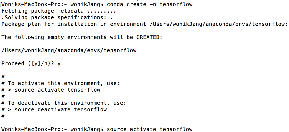
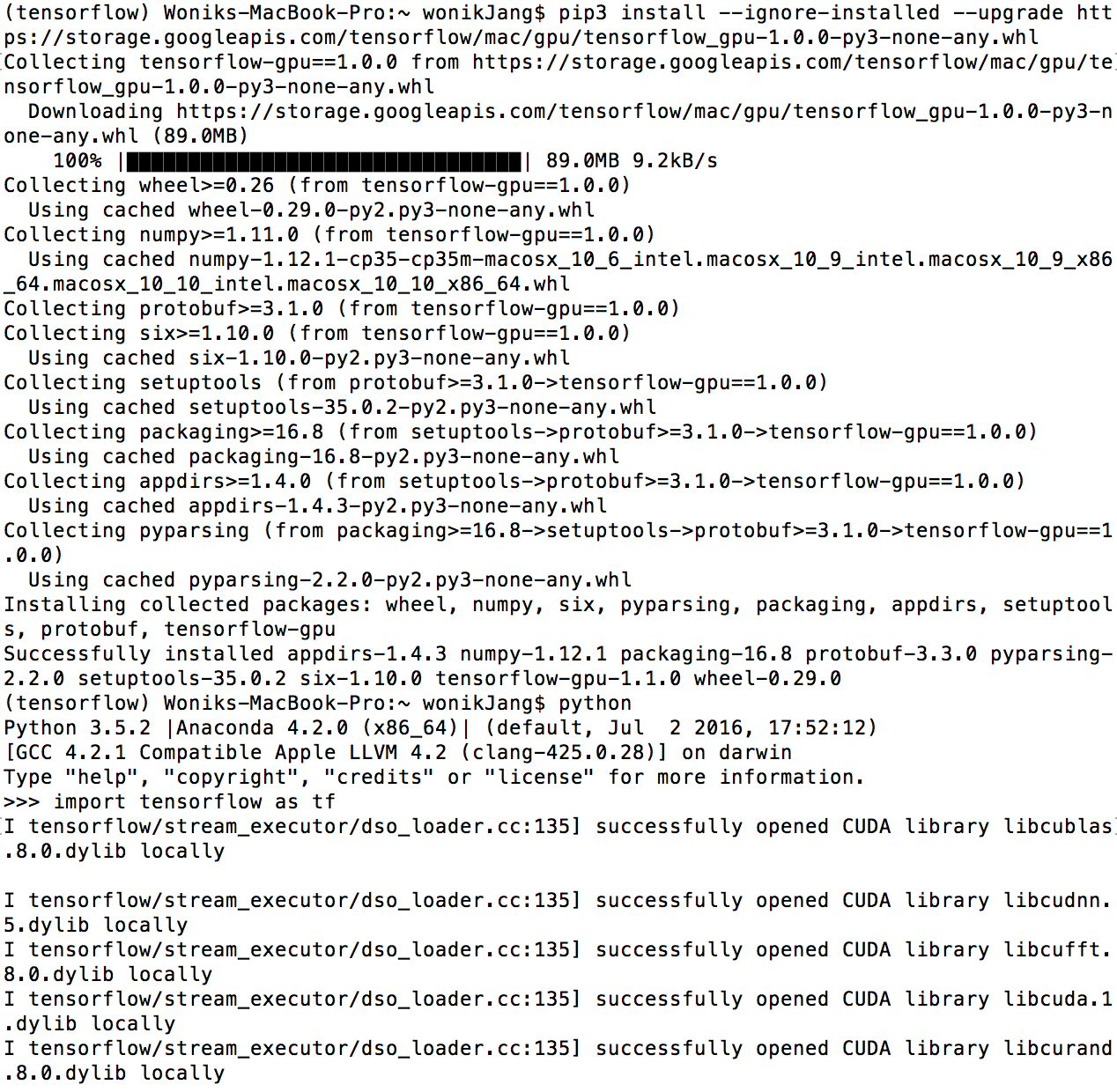
3 GPU, python version 3.4 or 3.5
pip3 install --ignore-installed --upgrade https://storage.googleapis.com/tensorflow/mac/gpu/tensorflow_gpu-1.0.0-py3-none-any.whlIn case of python 3.x, use pip3 instead of pip
(tensorflow)$ pip3 install --ignore installed --upgrade $TF_BINARY_URL4 Validate Tensorflow install
In terminal,
$ python>>> import tensorflow as tfImporting tensorlfow will show you comments like “successfully opened CUDA library libcudnn.5 dylib locally”
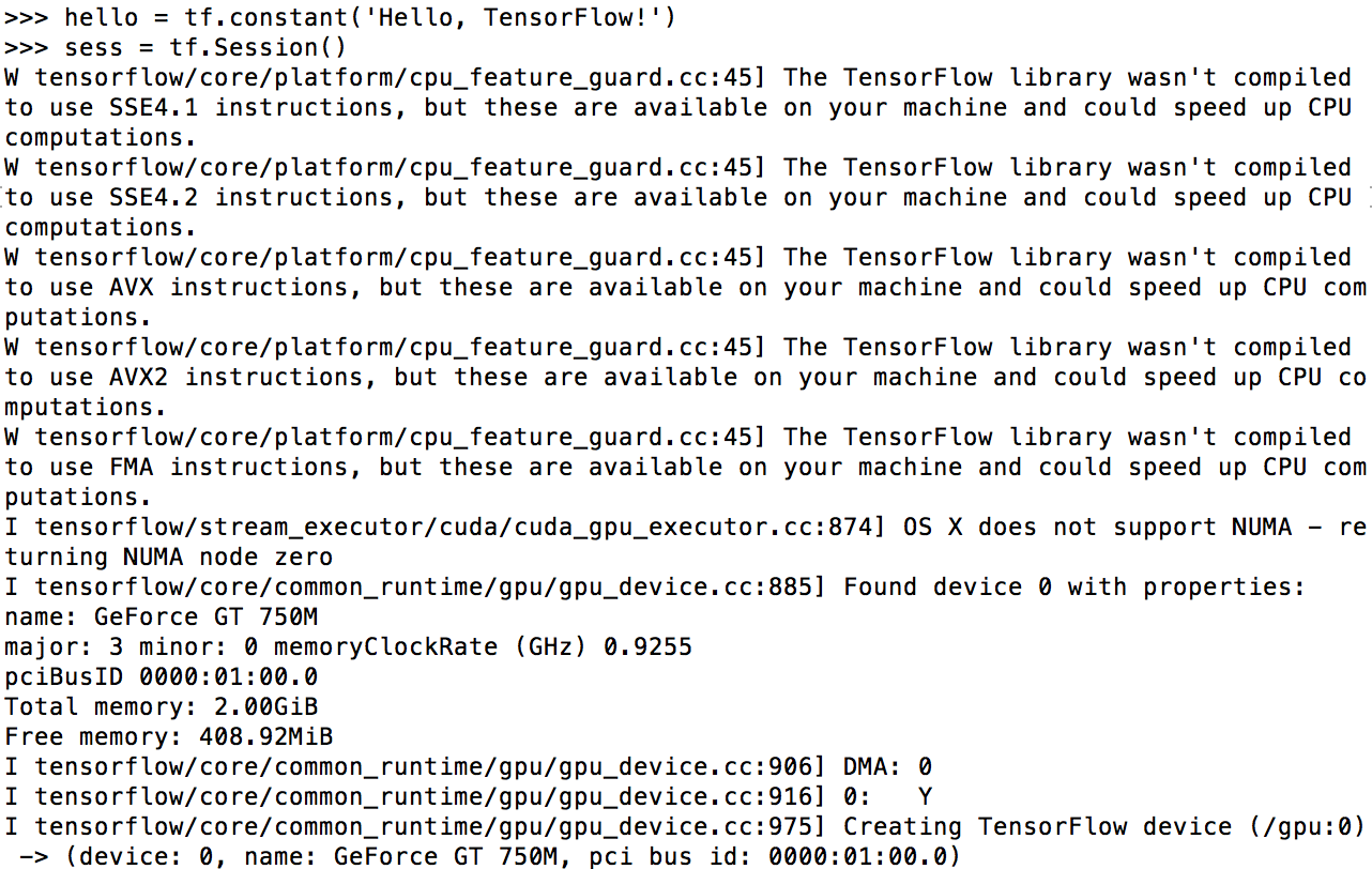
>>> hello = tf.constant('Hello, Tensorflow')
>>> sess = tf.Session()
>>> print(sess.run(hello))
Finally, you can figure out that total memory of GPU is loaded (In my case, 2GB)
If you encounter error message like below,
ImportError: No module name copyreg upgrade protobuf by typing
pip install --upgrade protobuf
